MDM4U - PROJECT BY SECTIONS
Normal Probability DistributionThe focus of the section on the Normal Probability Distribution is to identify
situations that give rise to Normal distributions by demonstrating an ability to
understand the properties of the Normal distribution, use these properties to
solve problems and make probability statements about Normal distributions.
The Normal Probability Distribution is a fundamental building block for most
elementary parametric Statistics, important applications are1. it is the theoretical distribution of random error when the scale is
continuous, for example, if every student in your school was given
a ten centimetre rule to measure the length of the gym, the
resulting distribution of their measurements would follow a Normal
distribution.
2. it is the theoretical distribution for the means of randomly drawn
large samples, for example, if everyone in the class rolled a dice
50 times and was asked to compute the mean of their results,
the distribution of the means from the class would follow a Normal
distribution.Area of Interest
Driver injuries and age group.Refined Question
Which age group has the most driver fatalities? Serious Injuries?Data
The Data used for this section has come from Canadian Motor Vehicle Traffic Collision Statistics 2000. (the website in the pdf file was http://www.tc.gc.ca/roadsafety).Analysis
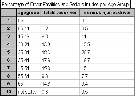
I have created a data chart containing data from the Canadian Motor Vehicle Traffic Collision Statistics 2000.
We can see that 25-34 year olds have the highest percentage of driver fatalities.
We can also see that 25-34 year olds also have the highest percentage of
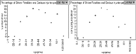
serious injuries.We can see that the above dot plots represent a bell shaped curve. The high
percentage value for 65+ is explained by the larger size of the age group. Notice
also that the grouping for ages 15-24 is divided into 15-19 and 20-24. We should
also notice that the age groupings do not all have the same range. I am allowing
this due to lack of normally distributed attributes concerning the section of the
transportation industry with an understanding that this will affect the probabilities
we will compute later. We will assume that these values represent a population
that has a normal distribution.To calculate the mean, µ , and the standard deviation, ó , we use the formulas:

Note: We will isolate our data to ages 5-64 to avoid an overly high mean due to
the jump of values at 65+. We will only be using m and s to create a hypothetical
set of values to use for problem solving.Driver Fatalities:
Driver with Serious Injuries:

Lets assume that the driver fatalities are normally distributed with mean 30.5 with
standard deviation 13.3. Lets assume that the driver serious injuries are normally
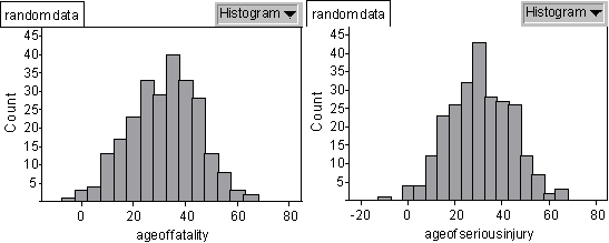
distributed with mean 31.2 with standard deviation 12.8. I will now use Fathom to
create a sample of 250 values for age of fatalities and 250 values for age of
serious injuries.
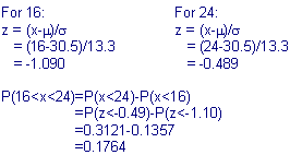
If the population is equal to 250 (let s ~= ó), what is the probability of a
driver who is killed is between 16 and 24 years old?
Therefore the probability a driver who is killed is between 16 and 24 years
of age is 17.64%.If we only have a sample of 250 people, what is the probability of a driver that
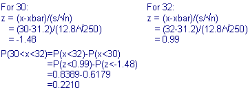
is seriously injured is between 30 and 32?
Therefore the probability of a driver that is seriously injured is between 30
and 32 is 22.1%.
What ages do 95% of driver fatalities occur?
Therefore 95% of driver fatalities occur between ages 17.7 and 43.3.Consider the youngest 63% of drivers with serious injuries. What is the oldest
driver with a serious injury?
We must find a corresponding z value to 0.63.
z=0.33
Therefore, concerning the youngest 63% of drivers with serious injuries, the
oldest would be 35.424 years old.Conclusion
I found that by using a modified x-axis (agegroup) I could use the data (mean and
standard deviation) from the Motor Vehicle Statistics, whose graph formed a bell
curve, to generate a hypothetical normal distribution to compare ages with
serious injuries and fatalities in automobile accidents. We then used the
properties of the normal distribution to solve problems relating to probabilities
concerning age andinjuries including death.Exploration
The Fathom Workshop Guide that I used in my exploration of simulation suggests
that the distribution of the mean proportion of males in my samples follows a
Normal distribution.Plan and Data
What I plan to do is to use the data generated from the simulation and to analyse
the distribution through the tools supplied by Fathom.Analysis
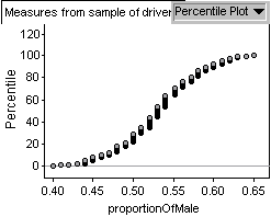
If the simulation data follows a Normal distribution I would expect the cumulative
distribution to look like an S shaped curve very similar to the one I obtained. I can
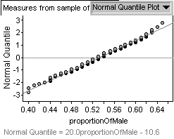
get better visual confirmation that the data follows a Normal distribution by
looking at the Normal Quartile Plot provided by Fathom.
From the Fathom Help file - A Normal Quartile Plot shows the distribution
continuous (numeric) data. It plots the z-scores associated with the percentile of
each case if the data were normally distributed. Therefore, if the data are
Normal, the plot should show a straight line. My simulation data is very close to
the straight line shown on the plot.Finally, I can do some checking whether the distribution of my simulation data
has the following properties of the Normal Probability distribution:
50% of the data falls on each side of the mean
About 68% of the data falls within one standard deviation of the mean
About 95% of the data falls within two standard deviations of the mean
About 99% of the data falls within three standard deviations of the mean
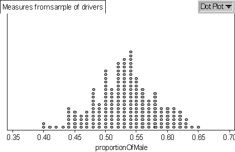
For my simulation data the mean proportion is 0.531, the standard deviation is 0.0497 and the Dot Plot is
where each dot represents two data. I counted the data in each interval and
divided by 200 hundred to get the percentage within each interval. I found the
percentage of data that falls on either side of the mean is 49.5% and 50.5%,
which is about 50% on each side of the mean.
The percentage of data that falls within one standard deviation (0.48 - 0.58) of
the mean is 73.5, which is larger than the predicted 68%.
The percentage of the data that falls within two standard deviations (0.43 - 0.63)
of the mean is 97%, which is larger than 95%.
The percentage of the data that falls within three standard deviations (0.38 -
0.68) of the mean is 100%.I did not have time to explore whether the approximations that I did (rounding off
the mean and standard deviation, and counting from the Dot Plot rather than
using the raw data) biased these results.Conclusion
The work that I did suggests that the distribution of the data I obtained from the
simulation could be modelled by the Normal probability distribution.Checklist
Student Name : _______________________________
Area Of Interest : ______________________________
Data to Normal Distribution
Normal DistributionProblems Solved Using
Normal Distribution
