Theory of Attitude Measurement
Louis L. Thurstone
University of Chicago
It is the purpose of this paper to describe a new psycho-physical method for measuring the psychological or functional similarity of attributes. Its development was motivated primarily for the solution of a particular problem in the measurement of social attitudes and it is in terms of this problem that the new psychophysical method will be described.
Let each of a group of N individuals be labeled as to the presence or absence of each of n attributes. This means that we are dealing with N persons and that each of these persons declares the presence or absence in him of each of the n, attributes. It does not matter for our present purposes whether the declarations are made by these people for them-selves or by others for them. In our particular problem we are dealing with a list of n statements of opinion and each person has the option of endorsing or rejecting each of the n opinions. The statement of an opinion is here regarded as a description of an attribute and the subject merely indicates whether he possesses the attribute. A similar analysis might be made for a series of traits which are supposed to describe people along an extroversion-introversion continuum, an ascendance-submission continuum, and so on. Our primary interest is here in the attitude continuum.
We postulate, for verification, an attitude continuum for the n opinions. Let them describe different attitudes toward the church for purposes of illustration. Some of the opinions reflect attitudes very favorable and loyal to the church; others are neutral or slightly favorable, while still others are slightly or strongly antagonistic to the church. We want an objective procedure for ascertaining whether any particular set of opinions really behaves as a continuum when the endorsements are analyzed.
( 223)
Let us consider first a pair of opinions, one of which is clearly favorable to the church and the other as clearly antagonistic.
1. I feel the church services give me inspiration and help to live up to my best during the following week.
2. I think the church seeks to impose a lot of worn-out dogmas and medieval superstitions.
Now, on a common sense basis, we should expect to find that of the people who endorse opinion 1 relatively few will endorse opinion 2. Similarly, those who endorse 2 will only seldom endorse 1. The following pair of opinions would probably behave differently.
1. I feel the church services give me inspiration and help to live up to my best during the following week.
3. I believe the church is the greatest influence for good government and right living.
If we consider the group of people who endorse 1 we should expect a rather high proportion also endorsing 3 because the two statements are both favorable to the church. The attitudes represented by these two statements may be expected to co-exist in the same person while 1 and 2 are more or less mutually exclusive.
These facts suggest the possibility of measuring the psycho-logical similarity of opinions in terms of the endorsements. For the two opinions we shall have the three following facts :
n(1) = the total number of individuals in the group N who endorse opinion No. 1.
n(2) = the total number of individuals in the group N who endorse opinion No. 2.
n(12) = the total number of individuals in the group N who endorse both 1 and 2.
Other things being equal, a relatively high value for n(12) means that the two statements are similar. A relatively low value for n(12) means that the two opinions are more or less mutually exclusive.
We shall avoid mere correlational procedures since it is possible in this case to do better than merely to correlate the
( 224) attributes. When a problem is so involved that no rational formulation is available, then some quantification is still possible by the calculation of coefficients of correlation or contingency and the like. But such statistical procedures constitute an acknowledgment of failure to rationalize the problem and to establish the functions that underlie the data. We want to measure the separation between the two opinions on the attitude continuum and we want to test the validity of the assumed continuum by means of its internal consistency. This can not be done if we had merely a set of correlational coefficients unless we could also know the functional relation between the correlation coefficient and the attitude separation, which it signifies. Such a function requires the rationalization of the problem and this might as well be done, if possible, directly without using the correlational coefficients as intermediaries.
Before summarizing these endorsement counts into an index of similarity we
shall introduce another attribute of the statement, namely, its reliability.
Suppose that there are N(1) individuals in the
experimental population whose attitudes toward the church are such that they
really should endorse statement 1 if they were conscientious and accurate and if
the statement of opinion were a perfect statement of the attitude that it is
intended to reflect. Now suppose that as a result of imperfections, obscurities,
or irrelevancies in the statement, and inaccuracy or carelessness of the
subjects, there are only n(1) endorsements of this
statement. Then the reliability of the opinion would be defined by the ratio

The notation pl means the probability that the statement will be endorsed by a subject who would endorse it if he were accurate and if the statement were a perfect expression of tilt attitude it is intended to convey. The question naturally arises as to how to ascertain the value of N1 which could be obtained directly only if the statement were perfect and the subjects absolutely accurate.
( 225)
We shall consider three methods of determining approximately the reliability of each statement.
1. Let the whole list of opinions be presented twice in random order. If there are fifty opinions in the experimental list there would be one hundred opinions to be read to the subjects, each opinion being repeated once. Let the endorsement counts for opinion 1 be as follows.
n1 = total number of subjects who endorse the first presentation of No. 1.
n1' = total number of subjects who endorse the second presentation of No. I.
n12 = total number of subjects who endorse both presentations of No.1.
The proportion of those who checked 1 who also checked 2 is

and we shall assume that this proportion is the same as the proportion of
those whose attitudes are of opinion 1 who actually checked that opinion. In
other words,
Similarly for the second presentation of the same opinion we have

But we can not expect the experimental values of n1' and n1' to be exactly the same so we shall use them both for determining the value of pl by the product of (2) and (3) so that
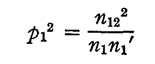
and hence

2. A second procedure which should give at least roughly
(226) comparable results is as follows. Let the entire list of opinions be sorted into any convenient number of groups by the method of equal appearing intervals. The statements may then be placed in rank order from those that are most antagonistic to the church to those that are most favorable. The detailed procedure for this scaling has been described elsewhere.[1] Then any two adjacent opinions will reflect practically the same attitude especially if the list is as long as 40 or 50 opinions or more over the whole available range of the attitude continuum.
Let any two adjacent opinions in this rank order series be numbered 1 and 2 respectively. The total number of individuals in the experimental population whose attitudes are represented approximately by the adjacent opinions 1 and 2 may be designated N12. If both of the statements were perfect and if the subjects were absolutely accurate, then we should expect to find n12 to be very nearly equal to N12, which is the full number of subjects whose attitudes are that of opinions 1 and 2. Strictly speaking, we are combining here two factors of reliability into one, namely the reliability of each opinion and the mean conscientiousness of the subjects. The reliability of the statement is the probability that a subject will endorse it if the subject's attitude is that of the opinion. It is a function of such characteristics of the statement as obscurity, subtlety or indirectness of its meaning, or actual ambiguity in its meaning. The reliability of the subject is the probability that he will endorse the opinions that he really should endorse in order truly to represent his attitude. This reliability is a function of such factors as the conscientiousness of the subject and the experimental arrangement. If the subject is asked to read several hundred statements of opinion he will not read them so carefully as if he is asked to read only a dozen. But we have combined these factors of reliability into a single index, the probability that the statement will be endorsed by the people who should
( 227) endorse it. If this type of analysis should prove to be fruitful there will no doubt be further investigations in which these factors of reliability are analyzed separately and explicitly.
Since there are N12 individuals who should check opinion 1 and
since the actual number who checked this opinion is only n1 the
probability that this statement will be endorsed by those who should endorse it
is
and, similarly,

These two probabilities are assumed to be practically uncorrelated so that

or

and hence

and

The assumption that the two probabilities of endorsement are uncorrelated is probably incorrect because the subject who is conscientious in reading one of these opinions will of course be likely to be conscientious also in reading the second opinion and consequently the probability that the two opinions will both be endorsed is not, strictly speaking, the product of the two separate reliabilities. The approximation is perhaps sufficient for our purposes and it may be hoped that it introduces no violent error.
The above procedure enables us to estimate the reliabilities of the opinions in terms of known data but this particular method requires that the opinions in the experimental list be first sorted into a rank order series by the method of equal appearing intervals or into a simple rank order series.
(228)
3. A third procedure is really identical with the second above except that instead of obtaining adjacent opinions by submitting the entire series of opinions to a large group for sorting, the experimenter selects adjacent statements by inspection. This is certainly not a safe procedure and it should be discouraged. A modification that could be acceptable is to select pairs of opinions that are paraphrased forms of the same statement, and then apply the logic of the second procedure above. It is by no means certain that these three methods of determining the reliability of a statement will give similar values. It might very well happen that the first procedure described above gives a measure of reliability in terms of factors more restricted than those which enter into the second and third procedures. If such is the case the first procedure gives values that are too high while the second and third procedures may give values more appropriate to our purposes.
We now have the following statistical facts about the two opinions whose separation on the attitude continuum is to be ascertained.
n1 = total number of individuals who endorsed opinion No. 1.
n2 = total number of individuals who endorsed opinion No. 2.
n12 = total number of individuals who endorsed both opinions.
p1 = reliability of opinion No. 1.
p2 = reliability of opinion No. 2
Let one of the opinions have its scale value at S1 on the attitude continuum of Fig. 1. Let there be N1 persons in the experimental group who should endorse it if they were absolutely accurate and if the statement of opinion were a perfect representation of the attitude it is intended to convey. The actual number of subjects who really do check this opinion is
n1= N1 p1,(11)
in which pi is the reliability of the statement.
( 229)
Now consider another statement whose scale value is at S2 on the attitude continuum. Since there is a difference (S2 — S1) between the attitudes of these two statements we should not expect all of the n1 subjects to endorse this second statement. If it were perfect in reliability, then the number of subjects in the group n1 who also endorse statement 2 will be
n1φ = N1p1φ (12)
where cp is some value less than unity. Now, it is reasonable to assume that if the two statements are far apart on the scale, then the proportion φ of the group n1 who also endorse the distant statement 2 will be small. This is represented in
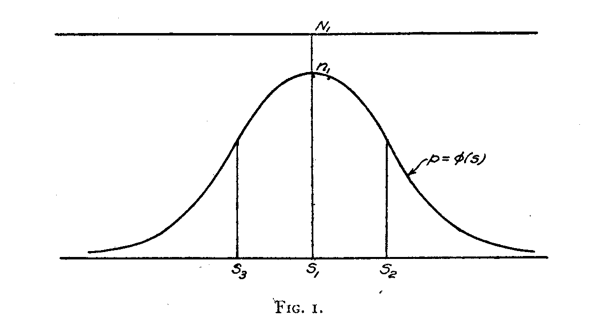
Fig. 1 by the fact that φ is a maximum when the separation (S2— Sl) is small while it approaches zero as this separation becomes large. We shall assume that this function is symmetrical about the axis at S1so that
P1(k) = φ(Sk – S1)2; (13)
in which p1(k) is the proportion of those who endorse statement 1 who also endorse statement k while Sk is the scale value of statement k. Our assumption is that pl(k) is a function of the separation (Sk- S1) but that it is independent of the sign of the separation which is an arbitrary matter.
We must also take into consideration the fact that statement 2 is probably imperfect as well as statement 1. Let its
(230) reliability be p2 and we shall then say that the number of those who check statement 1 who also check statement 2 is
n12 = n1φp2 = Nlplp2φ. (14)
The number of those who checked No. 1 who also checked No. 2 is of course the same as the number of those who checked No. 2 and who also checked No. 1. Hence, we may write, by analogy,
n12 = N2p1p2φ (15)
or
n12 = n1p2φ, (16)
n12 = n2p1φ,
and hence
n122 = p1p2n1n2φ2 (17)
or

This is the coefficient of similarity of two statements of opinion. When this value is relatively high, the two statements belong close together on the scale but when is small they are far apart.
This formula may be used to determine the reliabilities p1 and p2
if the two statements are known to have practically the same scale value. This
fact may be known either because of the fact that they are statements of the
same idea, one being a paraphrase of the other, or by being scaled by the method
of equal appearing intervals, previously described. Since the coefficient φ
deviates from unity supposedly only on account of the scale separations, it is
in this case unity, the two statements having practically the same scale value.
Then
But
N1 = N2,
since both of these symbols represent the same quantity, namely the number of people in the total group who should endorse both statements at the same scale value if both
( 231) statements were perfect. Hence

or
n1p2= p1n2 (21)
and

Substituting (22) in (19) we have

and hence

and, by analogy,

Our next problem concerns the exact formulation of the function
φ1k= f(Sk –S1)
We shall try first the assumption that it is Gaussian so that

This means that if a man has endorsed any particular perfect statement No. 1, the probability that he will also endorse another perfect statement No. 2, distant from No. 1 by the scale separation |S1 – S2|, is assumed to be a Gaussian function of the scale separation. This assumption can be tested empirically by the internal consistency of the scale, but the function can also be studied directly without this assumption by methods that will be left for separate publication. We shall assume for the present experiment that this φ-function has a maximum value of unity when the scale separation is zero.
(232)
We shall test the index of similarity on a set of ten statements of opinions selected at random from different parts of an attitude scale of 45 such statements. The random set of ten statements is less unwieldy to handle for illustrative purposes than the whole list of 45 in the church scale because the index involves a comparison of each statement with every other statement in the whole list. There will be therefore 10.9.1/2 = 45 comparisons for a set of 10 statements while there would be 45.44.1/2 = 990 comparisons necessary to handle the whole table of 45 statements.
The ten statements were selected so as to represent several degrees of attitude toward the church, including favorable, unfavorable, and indifferent opinions. Each statement is identified by a code number as follows :
2. I feel the church services give me inspiration and help to live up to my best during the following week.
4. I find the services of the church both restful and inspiring.
6. I believe in what the church teaches but with mental reservations.
11. I believe church membership is almost essential to living life at its best.
15. Sometimes I feel that the church and religion are necessary and sometimes I doubt it.
32. I believe in sincerity and goodness without any church ceremonies.
34.I think the organized church is an enemy of science and truth.
35.I believe the church is losing ground as education advances.
41. I think the church seeks to impose a lot of worn-out dogmas and medieval superstitions.
43.I like the ceremonies of my church but do not miss them much when I stay away.
In Table 1 we have all the necessary raw data. There are three types of fact here recorded: (i) The total number of individuals who endorsed each of the ten statements. These
( 233)
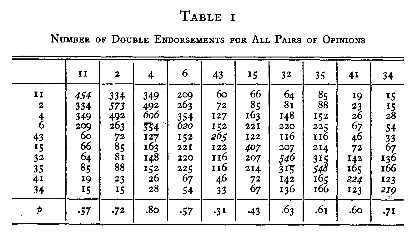
are found in the diagonal of the table. For example, there were 696 individuals who endorsed statement 4 in the total group of about 1,500 persons who filled in the complete attitude scale. (2) The total number of individuals who endorsed any particular statement and any other particular statement. These data are found in the body of the table. For example, there were 263 individuals who endorsed both statements 6 and 2. (3) The reliability of each of the ten statements. These are found in the last row of the table. They were determined by the second method described above which was applied to each of the statements in the whole scale of forty-five opinions. For example, the reliability of statement 32 is .63 which means that it was endorsed by 63% of the estimated number of people who should have endorsed it if the statement had been perfect and if the subjects had been perfect in their reading and endorsing.
In Table 2 we have listed the φ-values for all the comparisons. This is done by equation 18. The following is an example of the calculation of the φ-coefficient for the two statements 4 and 32 with data from Table 1.
It is seen that the table is symmetrical. The entries along
( 234) the diagonal are necessarily unity because there is of course no scale separation between a statement and itself. We shall now use these φ-values to measure the scale separation between all pairs of statements. This is done by entering an ordinary probability table with the values of φ in order to ascertain the deviation from the mean in terms of the standard
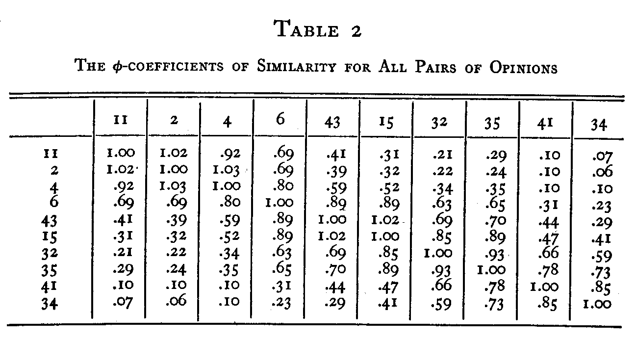
deviation of the assumed Gaussian function. Each of these deviations will be regarded tentatively as the scale separation between the two statements concerned. When the value of φ is small we shall therefore assign a rather large separation to the two statements. When the value of φ is high, near unity, we shall assign a rather small scale separation to the statements. It is more convenient for this problem to use a probability table in which the maximum ordinate is unity than to use a table in which the total area is unity so that the maximum ordinate is .4. It is also more convenient to use a probability table which is entered with the ordinate to ascertain the deviation rather than to use a table which is entered with deviations or proportions to ascertain the ordinates. The latter kind of probability table requires interpolation for this problem. The separation between statements 43 and 6 may be taken as an example. The φ -coefficient for these two statements is .89 as shown in Table 2. With this ordinate of the probability curve, the deviation is .48σ as recorded in Table 3.
(235)
The sign of the deviation is determined by the end of the scale which is arbitrarily called positive. In the present case the origin was arbitrarily placed at the opinion least favorable to the church namely statement 34. Therefore the statements favorable to the church are arbitrarily called positive with regard to the statements that are unfavorable to the church. It is entirely immaterial for scaling purposes which ends of the sequence of opinions are designated as positive and negative.
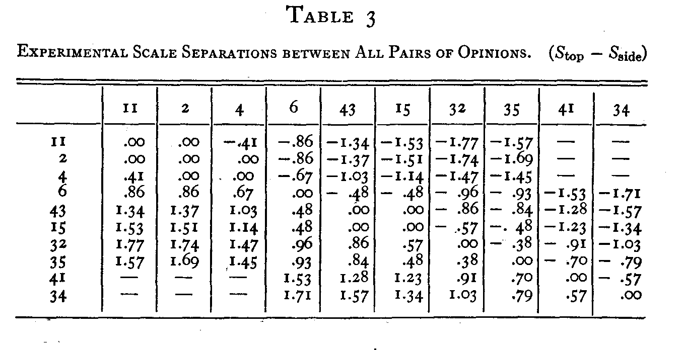
The signs in Table 3 are recorded so as to show (Stop – Sside). For example, the scale separation (S43 — S6) is found at the intersection of 43 at the top with 6 at the side. It is –.48σ. Similarly the separation (S6— S43) is found at the intersection of 6 at the top with 43 at the side. It is +.48σ. The two halves of the table are symmetrical about the diagonal of zero entries. The ten statements were arranged in Table 1 in order of scale values determined by the method of equal appearing intervals.[2] All separations as large as 2.σ or larger were ignored in Table 3 because when the separations become as large as that their reliabilities become too low to be acceptable. It is entirely arbitrary at what limit we shall drop the separations. They might be extended indefinitely if the
( 236) observations were weighted but that is too awkward. In these tables we have recorded separations only as large as 2.σ. There may also be some uncertainty as to how far the Gaussian curve can be used for the function φ = f (s) and this is another reason for not using scale separations larger than about 2.σ.
We are now ready to determine the average scale separation between successive statements in the present list of ten. It is done as follows:
Let Sl and S2 be the scale values of any two statements whose separation is to be measured. Then
x12 = (S1–S2) (27)
is a direct measurement of this separation which is obtained by the index of similarity φ12. This index is in turn a function of the raw data n1, n2, n12, p1, p2, so that

But we also have many indirect measurements of x12 which may be shown as follows.
Let Sk be the scale value of any other statement except 1 and and 2. Then
S1 – Sk = x1k
S2 – Sk = x2k
so that
S1 – S2 = x1k– x2k (29)
and hence

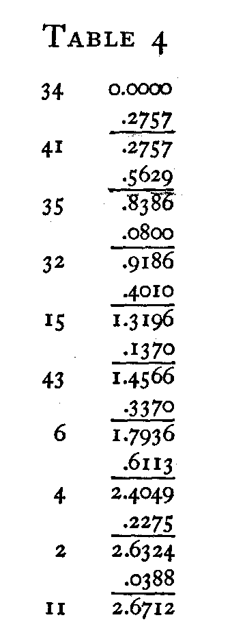
This equation is more accurate than (27) because it makes use of all the data in Table 1 while equation (27) makes use of only one of the φ-coefficients. Applying equation (30) to the data of Table 3 where n is in each of the nine successive comparisons the number of paired values, we obtain the successive scale separations shown in Table 4. We set the origin arbitrarily at statement 34 so that the final scale values from this
( 237) origin are as shown in Table 4. For example, the final scale separation between opinions 4 and 6 is obtained by equation 30. There are eight paired values for these two opinions in Table 3. The numerical values are as follows
Σx4k = + 5.35,n = 8,
Σx6k = + 0.46,S4 – S6 = + 0.6113.
Note that the sum Σx6k takes a different value when equation 30 is used to determine the scale separation between opinions 6 and 43 because there are then available ten paired values instead of eight for the interval 4 to 6.
We now want to test the internal consistency of our calculations. On the
basis of the final scale values of Table 4 we may construct a table of
calculated scale separations. This has been done in Table 5. For example, the
scale values of statements 43 and 35 are 1.46 and .84 respectively. Consequently
the calculated scale separation (S43 — S35) is + 0.62 as
recorded in Table 5, and the separation (S35 — S43) is the
same distance with sign reversed, namely – 0.62, also recorded in the same
table. The separations of Table 5 are based entirely on the ten scale values of
Table 4.
( 238)
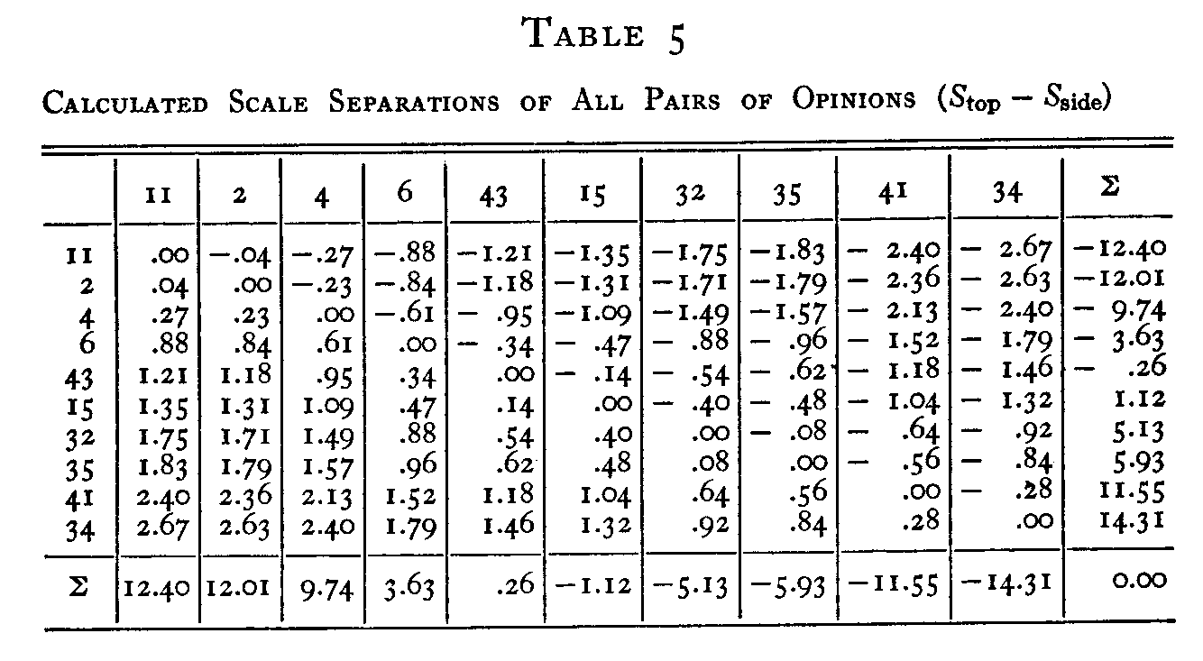
Now we want to know how closely these calculated scale separations of Table 5, based on the ten scale values, agree with the 45 experimentally independent scale separations of Table 3. The discrepancies between Tables 3 and 5 are listed individually in Table 6. The discrepancies between the
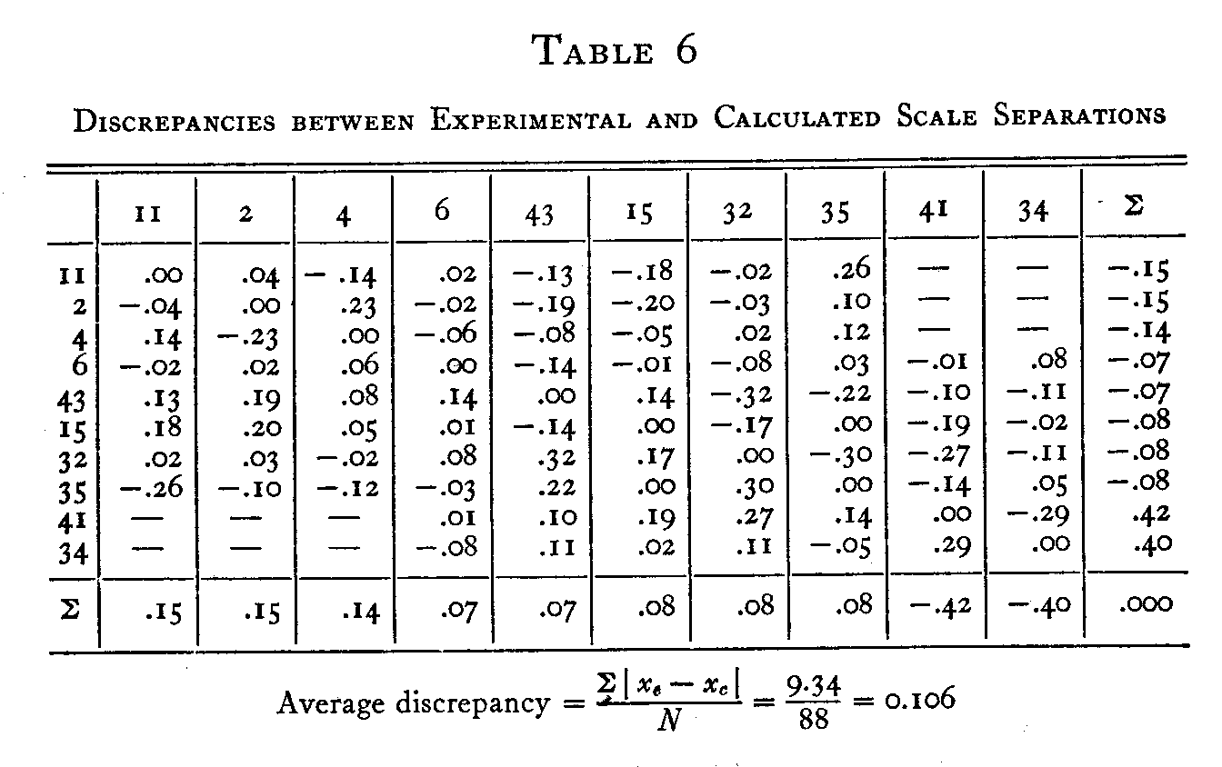
experimental and the calculated scale separations in Table t vary between zero and .32σ with a mean discrepancy of only .106σ. This mean discrepancy is only about 1-25 or 4 percent of the range of the scale values, 2.67σ, for the ten statements.
(239) Another set of ten statements, also selected at random from the entire list, has been subjected to the same analysis with comparable results.
The question might be raised why we have not used correlational coefficients instead of the 0-coefficient here de-scribed. Dissimilarity can of course be indicated merely by a correlational index or by contingency methods. Such indices do not constitute measurement except by a generous interpretation of the word measurement. We have attempted truly to measure degree of functional dissimilarity of two attributes or reactions. In order to satisfy what seems to be a fundamental requirement of measurement it is reasonable to expect that if the difference between two entities a and b is, let us say, plus five units, and if the difference between two entities b and c is, let us say, plus three units, then the difference between the two entities a and c should be the. sum of these two differences, namely, plus eight units, if all three quantities really measure the same attribute.
This simple requirement is not satisfied by correlational coefficients. If the correlation between a and b is .80 and that of b and c is .40 it does not follow that the correlation between a and c is some additive function of these coefficients. We have postulated a continuum, the attitude scale, and we want to measure separations between points on this continuum so that our measurements are internally consistent; so that (a – b) + (b – c) = (a – c) but such consistency is not found by correlational procedures.
Let it be desired to measure the areas of a lot of circles. Let the diameter of each circle be used as an index of area. It is now possible to arrange the circles in rank order according to area by means of the diameter-index. It is also possible to say of two circles that they must have the same areas because their diameters are equal, but these diameter measurements are hardly to be called measurements of areas. Equal increments of the diameter-index do not correspond to equal increments of what we set out to measure, namely area. The unit of measurement of the diameter does not correspond to a constant increment of area. All of this is childishly simple
( 240) but the reasoning is the same as regards correlational coefficients. They are not measures of dissimilarity. They are merely numerical indices of dissimilarity. In fact, correlation coefficients are what one resorts to in the absence of hypothesis and rational formulation. If the problem admits of rational formulation, then that function should be written and tested directly by experiment. If the problem is so complex that it defies analysis we can still correlate the variables and represent by correlation coefficients the degree of association between them. That is better than nothing, but it is not really measurement by our simple criteria. These considerations have led me to regard correlation coefficients as symbols of defeat. They constitute a challenge to try again and to outgrow the necessity for using them.
My efforts recently in psychological measurement have been to define in every case a continuum, to allocate people, tasks, and other entities to the continuum under investigation, and to check its validity by the simple criteria that have just been described. I believe that such efforts will prove more fruitful for psychological theory than merely to correlate everything with everything else under heaven.
The results of our attempt to construct an attitude continuum are shown graphically in Fig. 2, in which the ten

opinions are shown with their allocations to the attitude scale. An actual scale for measuring attitude should contain many more opinions and they should be so selected that they constitute as far as possible an evenly graduated scale. The church scale previously referred to has 45 opinions which have been selected from a list of 130 so as to constitute an evenly graduated scale. Our present purpose has been to show how the method of similar reactions enables us to construct such a scale from the records of endorsements. It is hoped that the
( 241) method may also prove useful as an objective test for the validity of other concepts such as extroversion-introversion, ascendance-submission, and the like.
SUMMARY
We have developed a new psychophysical method for measuring the psychological dissimilarity of attributes. This method assumes that if two attributes tend to coexist in the same individual they are regarded as functionally similar while if they are more or less mutually exclusive so that they tend not to coexist in the same individual, then they are functionally dissimilar. The degree of similarity is measured in terms of the 0-coefficient which enables us to allocate the attributes along a single continuum, and to measure the degree of similarity by scale separations on this continuum or scale. The method may be called a method of similar attributes or a method of similar reactions.
The φ-coefficient enables us to ascertain whether a series of attributes really belong functionally on the same continuum. This is done by the test of internal consistency as shown in Table 6. The method has been applied to the record of endorsements of 1500 people to ten statements of opinion about the church. It has been shown that these opinions can be allocated to a single continuum with measured scale separations. It has been the purpose of this study to make a rational formulation for the association of attributes by which the existence of continuity in a series of attributes may be experimentally established and by which their functional dissimilarities, the scale separations, may be truly measured. For these purposes correlational procedures are inadequate because correlational coefficients are not measurements.
[MS. received October 29, 1928]