The Method of Paired Comparisons for Social Values
L. L. Thurstone
University of Chicago and Institute for Juvenile Research
THIS is an attempt to apply the ideas of psychophysical measurement in the field of social values. Some of the psychophysical methods have been applied in a crude way to the measurement of educational products such as handwriting and English composition, and it seems feasible to apply the same ideas as well to social values although the attempt cannot readily be made without making compromises that the psychophysicist would not tolerate. The application of the principles of psychophysical measurement to educational products has been made with more or less similar logical handicaps but these do not seem to have disturbed the popularity of these methods in the field of educational measurement. Since the final results show a rather satisfactory internal consistency, one may possibly assume that the methods, the theoretically imperfect, have some value also in social psychology.
For the present experiment the seriousness of different crimes or offenses was chosen for such measurement. The seriousness of an offense we shall assume to be the seriousness as judged rather than as measured in terms of objective consequences or in some normative way. It may very well be that the relative seriousness of offenses, as judged by a group of individuals, may be quite wrong when looked at from the standpoint of objective checks or standards, but we shall be concerned here with the relative seriousness as judged by a group of several hundred students. These records we shall use for the purpose of ascertaining how the offenses arrange themselves in a quantitative continuum from those that seem to be most serious to those that seem relatively least objectionable. There is no doubt but that we imply such a continuum of seriousness in speaking about offenses. In fact we are supposed to regulate punishment more or less in accordance
( 385) with the seriousness of the offense. Is it possible to reduce these qualitative judgments about relative seriousness of different offenses to a quantitative basis?
The main principle that underlies the measurements in this study may be stated very briefly. Suppose that 90 per cent of the judges say that crime A is worse than crime B and that the remaining 10 per cent vote that B is the more serious. Now suppose, further, that 55 per cent, barely more than half of the judges, say that crime B is more serious than crime C. Then we should be justified in saying that the separation between the two offenses A and B on a scale of seriousness is much greater than the separation between B and C on that same scale. We might be able to talk even sensibly about "distances" on a scale of seriousness of crime. Some of these distances or separations are then to be considered greater than others. There is really nothing in common sense ;judgments that would be violated in such an analysis. Common qualitative judgment would probably be to the effect that murder, for example, is very much more serious than smuggling, and that there is not so much difference between smuggling and bootlegging. Some of us may individually disagree but the above comparisons would probably be true for most people. The present experiments constitute an attempt to measure these relative differences and to indicate one possible procedure in extending at least some of the ideas of psychophysical measurement to social values.
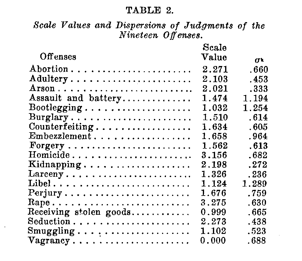
The following is a list of the nineteen offenses that were judged in these experiments.
| Abortion Adultery Arson Assault and Battery Bootlegging Burglary Counterfeiting Embezzlement Forgery Homocide |
Kidnapping Larceny Libel Perjury Rape Receiving stolen goods Seduction Smuggling Vagrancy |
The offenses were arranged in pairs so that every one of them was paired with every other one. The total number of pairs of offenses presented was therefore n (n - 1) /2 = 171.
The instructions to the subjects were as follows:
(386) The purpose of this study is to ascertain the opinions of several groups of people about crimes. The following list of crimes has been arranged in pairs. You will please decide which of each pair you think more serious and underline it.
An example: Cheating—Murder
You would probably decide that murder is a more serious offense than cheating, therefore you would underline murder.
If you find a pair of crimes that seen equally serious, or equally inoffensive, be sure to underline one of then anyway, even if you have to make a sort of guess. Be sure to underline one in each pair.
Receiving stolen goods—Perjury
Kidnapping—Adultery
Abortion—Libel
Burglary—Counterfeiting
Bootlegging—Arson
The remainder of the 171 pairs of offenses were presented in the same manner.
In the preliminary experiments it was found that some of the college students were unfamiliar with some of the terms and it was therefore necessary to supply a sheet of brief definitions. All of the subjects whose records are here reported were supplied with such a list of definitions.
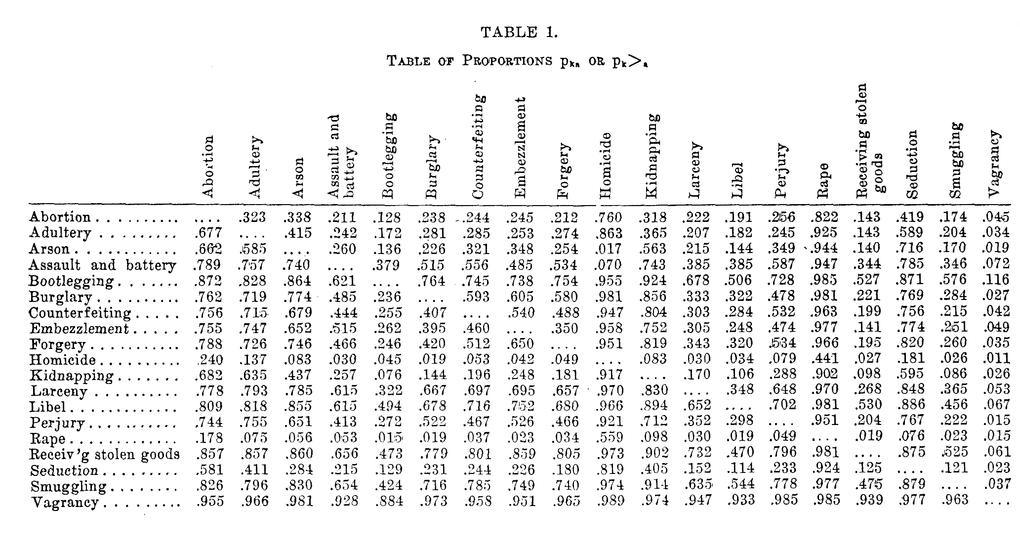
The lists of pairs of offenses were given to 266 students at the University of Chicago and the returns were practically complete. When the tabulations were made it was found that the number of omissions did not exceed five for any pair of offenses for the 266 subjects. The exact number of subjects who checked each side of each pair was tabulated and from these figures the proportions of Table 1 were calculated. Table 1 is to be read as follows. In any column such as that for forgery the records indicate the proportion of subjects who regarded forgery as more serious than the offenses listed in the left column. For example, if we compare forgery with bootlegging, we find in the table that 75.4 per cent of the students considered forgery more serious than bootlegging. If we look in the column for bootlegging we find that the complementary proportion, 24.6 per cent, considered bootlegging more serious than forgery. Such information is available in Table 1 for all the possible pairs of offenses.
The problem to be solved now is that of constructing a scale for the measurement of the seriousness of these offenses in the minds of the 266 students who served as subjects. Our raw data consist in the original frequency tables of checks and the resulting propor-
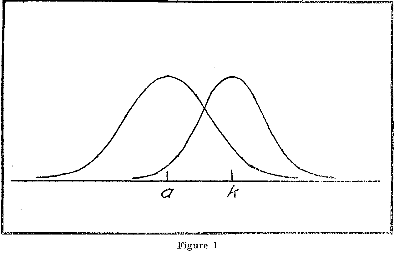
( 387) -tions in Table 1. Assume that the base line of Figure 1 represents the scale that we are seeking to establish. Let a be any one of the offenses that we choose to use as a standard, more or less as we should choose a standard in the method of right and wrong cases. Let k be any one of the other offenses which is being compared with the standard offense a. These two offenses, k and a, are of course separated by some unknown distance on the scale.
At this point it is of some interest to note a contrast between the scaling problem and the conventional psychophysical problem.
In psychophysics we take for granted that we know the stimulus intensities and we seek the proportion of correct judgments for varying stimulus differences. On the basis of such data 1w-e determine the standard deviation of the psychometric function and the stimulus value which corresponds to the origin of that curve. In the scaling problem the situation is more or less reversed. We are seeking to determine the stimulus values themselves. It is clear
that the scaling problem is much the more difficult, theoretically, because on the basis of the proportions such as those of Table 1 we seek to determine the stimulus intensities and the coarseness of discrimination, whereas the psychophysical problem is concerned only with the coarseness of discrimination while the stimulus intensities are known. The constant errors occur in both problems.
( 388)
Let us assume first that we are dealing with one subject who would repeatedly check the list of pairs of offenses according to the same instructions. The particular offense k would then on some occasions seem to him a little more serious than ordinarily, while on other occasions lie would judge that particular offense more leniently. It is probable that he would never judge the offense k a whole scale above or below its average value whereas small fluctuations in apparent seriousness would be very common. Here we shall assume that these fluctuations follow the laws of probability but we shall not be entirely satisfied to make this common assumption without some experimental check on its approximate validity.
We shall have then in Figure 1 a scale of seriousness of offenses with the offenses k and a hypothetically located thereon. We shall also assume that each offense is perceived with a certain standard error of observation. These standard errors of observation we shall designate sk and sa respectively. Now it is necessary to remind oneself that every single judgment "k is greater than a" or "k is less than a" involves the perception, recognition, or cognitive placement of, not one, but two entities, k and a. Hence every psychophysical judgment is the product of two errors of observation, one observational error for the standard and another observational error for the comparison stimulus. This fact is not generally acknowledged in psychophysical theory, and it is usually ignored entirely in educational measurement. As we have drawn the distributions of observational errors in Figure 1, it sometimes happens that k is perceived at low values, even lower than the average for a, and similarly it happens that a is perceived sometimes even higher than the scale value of k. If we take any pair of these observations of k and a, we shall find that k is usually perceived worse or stronger than a but the perceived difference (k1- a1) is sometimes negative. When k is perceived as stronger than a the perceived difference (k1- a1) is positive, and when k is perceived as less serious or weaker than a, then the perceived difference (k1- a1) is negative.
If we were able to plot a distribution of the perceived differences we should have a distribution like that of Figure 2. The base line in this figure represents the perceived difference (k1- a1). To the right of the origin on the base line these differences are positive and the corresponding ordinates of the frequency curve represent the relative expected frequencies of such perceived differences. The most common perceived difference is assumed to be the true
( 389) difference (k - a) and its frequency ordinate is therefore highest. To the left of the origin on the base line the differences are negative; in other words, that section of the base line represents perceived differences in which a is judged to be more severe than k. The standard deviation of this curve is a function of the two standard errors of observation for the two stimuli separately perceived and indicated in Figure 1. It is clear that the area of the
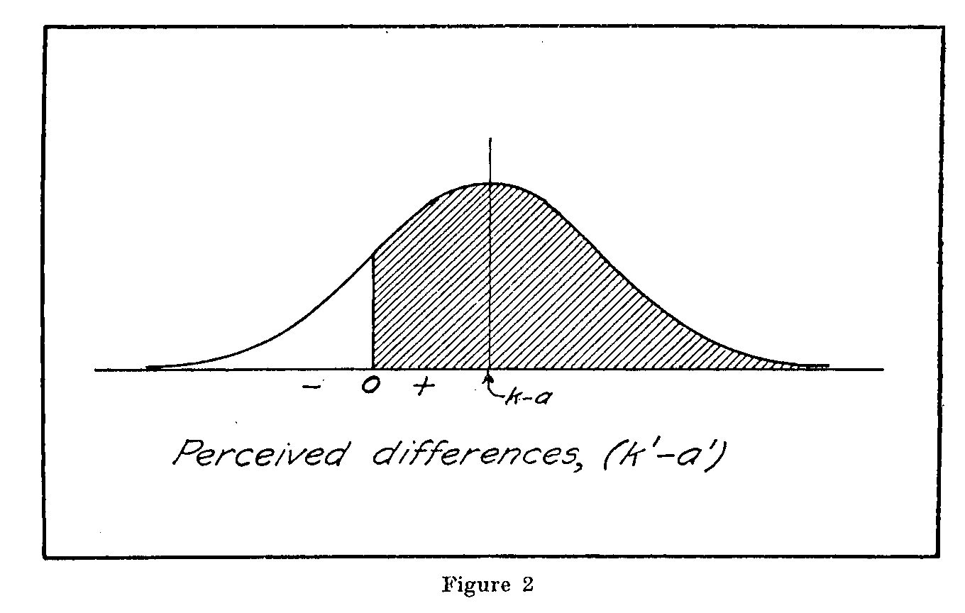
probability curve in Figure 2 represents the total number of judgments. The shaded area to the right of the origin represents that portion of the judgments in which (k1- a1) is positive while the unshaded remaining area represents the portion of judgments in which a is judged worse or stronger than k.
So far we have considered the judgments as though they had been made by a single observer repeating his judgments several hundred times. But our data actually involve such judgments, one set from each observer, for 266 subjects. This is a weak point in the argument in that we shall assume that the seriousness of a particular offense has some unmeasured relative mean value for all the subjects, and that the extreme judgments about its seriousness are less common than judgments at or near the unmeasured mean degree of seriousness for the whole group. That this assumption is not altogether unreasonable is indicated by two facts, namely that the proportions in Table 1 for any two standards, i.e., any two
( 390) columns in the table, do not give a linear plot, as they should do if we were dealing with rectangular distributions of judgments of seriousness. The second and more convincing fact is that the final scale values enable us to compare the theoretical with the actually observed proportions of judgments and these two sets of proportions for any given offense as a standard do give a fairly good linear plot as will be demonstrated later.
In Figure 2 we have, then, the theoretical distribution of perceived differences (k1- a1) and if the two stimuli, which are offenses in this case, are sufficiently close together these differences will sometimes be positive and sometimes negative. The mean of this distribution represents the most commonly perceived difference which may be assumed to be the true difference. The shaded area represents the proportion of perceived positive differences in which k is ,judged greater or stronger than a. That area is the theoretical or expected proportion of judgments "k worse or stronger than a". But this proportion is the one which is experimentally given for all pairs of stimuli in Table 1. Hence our problem is to determine those relative scale values a, b, c,---k, and those standard errors of observation sa, sb, sc, — sk which will best satisfy the experimentally observed proportions in Table 1. We shall then apply certain tests to ascertain- whether our results contain sufficient internal consistency to warrant acceptance of the procedure.
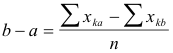
In Figure 2 let the shaded area be represented by pka. The area or proportion between the origin and the point (k - a) is therefore pka —.50. The relation between the theoretical distribution and the experimentally obtained proportions is given by the following equation:
| (1) | |
|
|
(2) |
in which
(k - a) is the distance on the base line between the origin of the curve and the mean ordinate.
xka= the deviation (k -a) in terms of the standard deviation. It is ascertained from the probability tables by means of the observed proportion pka.
ska =the standard deviation of the distribution of perceived differences for the two stimuli k and a.
Since the scale values of the offenses will be obtained by a process of summation it may be an acceptable approximation to assume all of the standard errors of observation, ska as equal. This approximation is not theoretically satisfactory but the solu-
( 391) -tion of the problem without this assumption becomes prohibitive and unwieldy. It probably does not affect the scale values seriously because these are to be determined by an arithmetical summation method in which all of these standard errors of observation are involved.
Let the standard errors of observation be designated ska and assume that they are all equal. Then, considering a as a standard stimulus and k as the variable stimulus,
| (2) | |
|
(3) |
and, by symmetry, using stimulus b as a standard instead of a,
![]()
But, by assumption,
![]()
Hence,
|
|
(3) |
From the two equations (3) we get
Let ska, be the unit of measurement for the scale. Then
|
(4) |
Hence it follows that the scale values, assuming that the errors of observation are identical for all of the stimuli, will he given directly by the following, relations, the signs obtained from equation (4) being arbitrary.
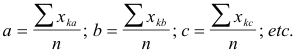
|
(5) |
In order to obtain the scale values of the offenses by equations 5, a table was prepared showing the value of x for each proportion. This table corresponds exactly to Table 1 except that instead of listing the proportions directly, these were translated
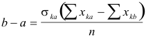
( 392) into their equivalent deviations in terms of their respective standard errors of observation. The table was obtained directly from Kelley's probability tables and the values Sxka, Sxkb, Sxkc, etc., were obtained as summations of the columns.
In order to make the scale values all positive an arbitrary origin was located at the offense which was judged least serious, namely vagrancy. The other offenses are scaled with that offense as a datum. The unit of measurement for the scale is the standard error of observation, ska, which is assumed to be constant for all of the offenses. This unit of measurement is theoretically 1.42 sa. In other words the standard error of observation for any pair of stimuli is always greater than the standard error of observation for either of the stimuli observed separately. The standard error of observation for any single stimulus is a subjective intensity distance which can never be directly measured by any objective means. It can, however, be indirectly determined.
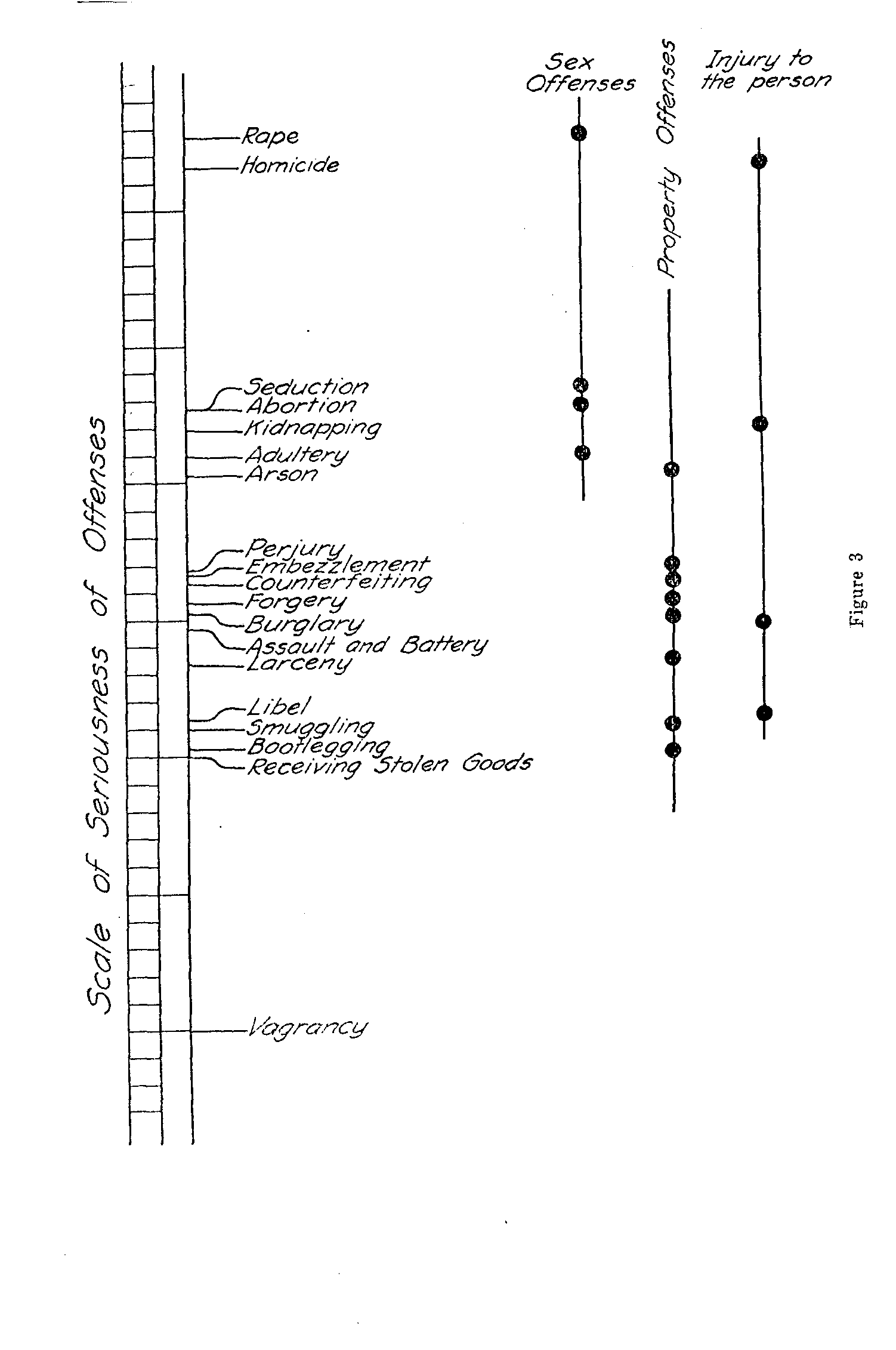
In Figure 3 the scale values of the offenses are represented graphically. Numerical designations on the scale are intentionally omitted. The scale values were determined from equations 5. The small circles represent the same scale values for offenses classified in groups. It is of some interest to note that all of the four sex offenses which were included in the list were judged to be more serious than all of the property offenses. In the minds of the 266 college students none of the property offenses was considered to be as serious as any of the sex offenses. There is no overlapping on the scale of sex offenses and the property offenses.
Another observation of some interest is the comparison of the two offenses which were judged to be most serious, namely rape and homicide. In the direct comparison of these two offenses in Table 1, 56 per cent of the subjects rated homicide as the more serious. But when the scale values of these two offenses are determined by the independent comparison with the other offenses, rape comes to the top as the more serious. The latter judgment is the indirect one obtained by comparing the scaling of the two offenses, not directly with each other, but by comparing their respective scaling with other offenses. The variation may, of course, be due merely to unreliability of the data.
Before we can test the internal consistency of the scale values just obtained it is necessary to calculate, at least approximately, the standard errors of observation for each of the offenses. In doing this we shall of course not make the assumption that they are all equal, an. assumption that we found convenient in the sum-
( 393)
( 394) -mation procedure for determining the scale values themselves. We start again with equation (1) which can be rewritten in the form
If stimulus a is the standard in this equation we can write (n -1) similar equations with the same standard since there are n stimuli in the series. The summation of these (it-1) equations takes the form
 |
(6) |
in which the notation mk, is adopted for convenience.
All of the (n -1) equations summed in equation (6) have stimulus a as a standard. A similar summation equation may be written for the (n-1) equations which have b as a standard, and so on for each of the k, stimuli. These it summation equations may be represented as follows:
|
(6) |
|
|
|
|
| . . . . . . . . . . . . . . . . . . . . . . . . . . . . . . . . . . . . . . | |
|
|
|
| |
(7) |
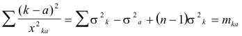
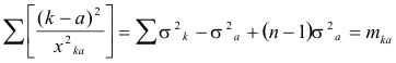
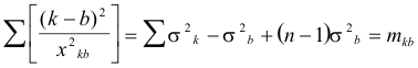
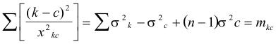
The notation M for Smkk is also used for convenience. From equation (7) we may determine the sum of the standard errors of observation for all of the nineteen offenses. This sum will be used in determining the separate standard errors of observation for each of the offenses.
In making the calculation of Ss2k tabulation is made of
( 395) (k-a)2 from the scale values and of x2ka from the deviations determined from Table 1. The summation
is then determined numerically for the eighteen values with offense a as a standard. The other eighteen summations corresponding to equation (6) are made in a similar manner. The total sum of these nineteen numerical values gives M which is used in equation (7) to determine Ss2k for all of the nineteen offenses.
The individual standard errors of observation are obtained from equation (6) in the following manner:
 |
(6) |
 |
(8) |
By means of equation (8) one may determine the individual standard errors of observation. These are summarized in Table 2.
The final test of internal consistency is to calculate the expected proportions of judgments "k>a" and to compare these calculated proportions with the actually obtained proportions. This can readily be done by means of the original equation (1) since we have assigned scale values a, b, c, — k, and the corresponding standard errors of observation, listed in Table 2.
For example, if Ave wish to predict from the scale values ,111d their corresponding errors of observation in Table 2 the proportion of the subjects who would rate seduction as a more serious mu offense than forgery, we should use equation (1) as follows:
| Scale Value | sk | |||
| Seduction | 2.273 | .438 | ||
| Forgery | 1.562 | .613 |
With these data from Table 2 we determine the value of from equation (1) and we find it to be +.94. This corresponds to a proportion of 83 per cent as determined by Kelley's tables. In other words, we should expect 83 per cent of the 266 students to say that seduction is a worse offense than forgery. In the experimental results of Table 1 we find that the actual proportion was 82 per cent. In many of the comparisons between the calculated and the experimental results the correspondence is even closer
(396) while in some of them the discrepancy is as much as 6 or 7 per cent, with an occasional discrepancy of 8 or 9 per cent. This correspondence is as close as may be expected from proportions based on 266 subjects.
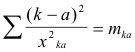
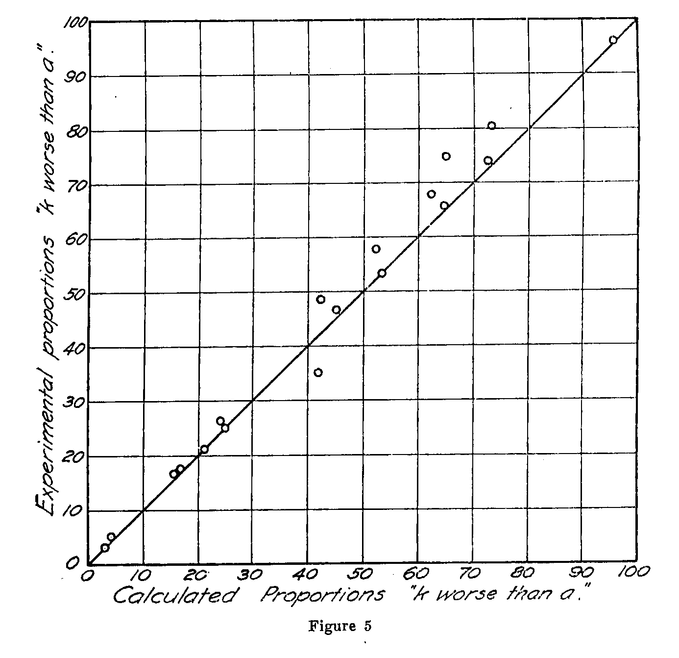
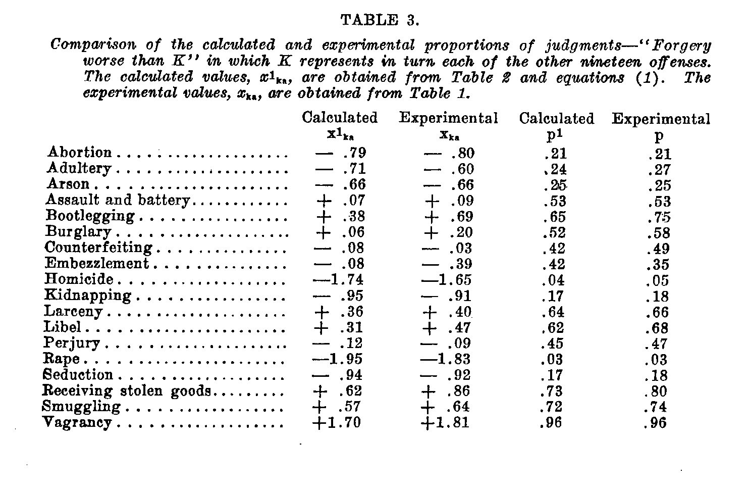
Such comparisons for isolated pairs of offenses in the list are not satisfactory as a check of internal consistency. It is better to compare the calculated and experimental proportions for all of the offenses with each one in succession as a standard. In Table 3 such a set of comparisons has been tabulated for forgery as a standard. These calculated data are obtained by means of equation (1). A similar table can be easily prepared for any of the other offenses as a standard. The table gives the calculated and experimental proportions of the 266 subjects who considered
( 397) forgery to be worse than each of the offenses listed. It also gives the corresponding sigma values. In Figures 4 and 5 these results are represented in graphical form. Since the fit is a fairly good one, we can assume that the original equation (1) is a satisfactory statement of the discriminatory judgments of the seriousness of the offenses.
SUMMARY OF THE METHOD
The stimuli whose magnitudes are to be measured are presented to the subject in paired comparisons. For each comparison he decides which of the two is the stronger. It is assumed that each of the stimuli has an unknown mean magnitude for the group and that there is a standard error of observation for each stimulus. Every judgment is assumed to be the result of four determinable
(398) factors, namely, the two stimulus magnitudes and the two standard errors of observation. The proportions of judgments are expressed in equation (1) as a function of these four factors. The experimental data consist in the observed proportions of judgments and from these data the best fitting scale values of the stimuli as well as their respective observational standard errors are determined.
A table of proportions like Table 1 is first prepared which summarizes the experimental data. A corresponding table of signa values is then prepared, in which the experimental proportions, represented by the shaded area of Figure 2, are expressed in terms of the deviation (k - a). The scale values of the stimuli are then determined by equations (5) on the assumption that the observational errors are approximately equal.
The sum or the standard errors of observation are then determined from equations (6) and equation (7). The individual standard error of observation for each stimulus is then calculated from equation (8). The internal consistency of the determinations is ascertained by comparing the experimental proportions with the calculated proportions by inspecting the goodness of fit for either of the procedures shown in Figure 4 or Figure 5.
The present study does not have for its purpose the discovery of any startling facts with regard to crime. It does show that qualitative judgments of a rather intangible sort, loaded usually with personal opinion, bias, and even strong feeling, and regarded generally as the direct antithesis of quantitative measurement, are nevertheless amenable to the type of quantitative analysis which is associated historically with psychophysics. It is of some interest to see that a set of numerical values can be established by which the 171 observed proportions of judgments about crimes and offenses can be summarized in generalized form.
(
399)
( 400)
|
|
 |