Mental and Social Measurements
Chapter 8: The Transmutation of Measures by Relative Position into Measures
in Units of Amount
Edward L. Thorndike
� 22. Transmutation by Means of Knowledge of the Form of the Distribution
FOR the sake of simplicity, only the case of individuals measured by their relative position in a group will be discussed in this chapter. The theory and technique described apply equally to any series of facts ranked in order for their amounts of any one trait.
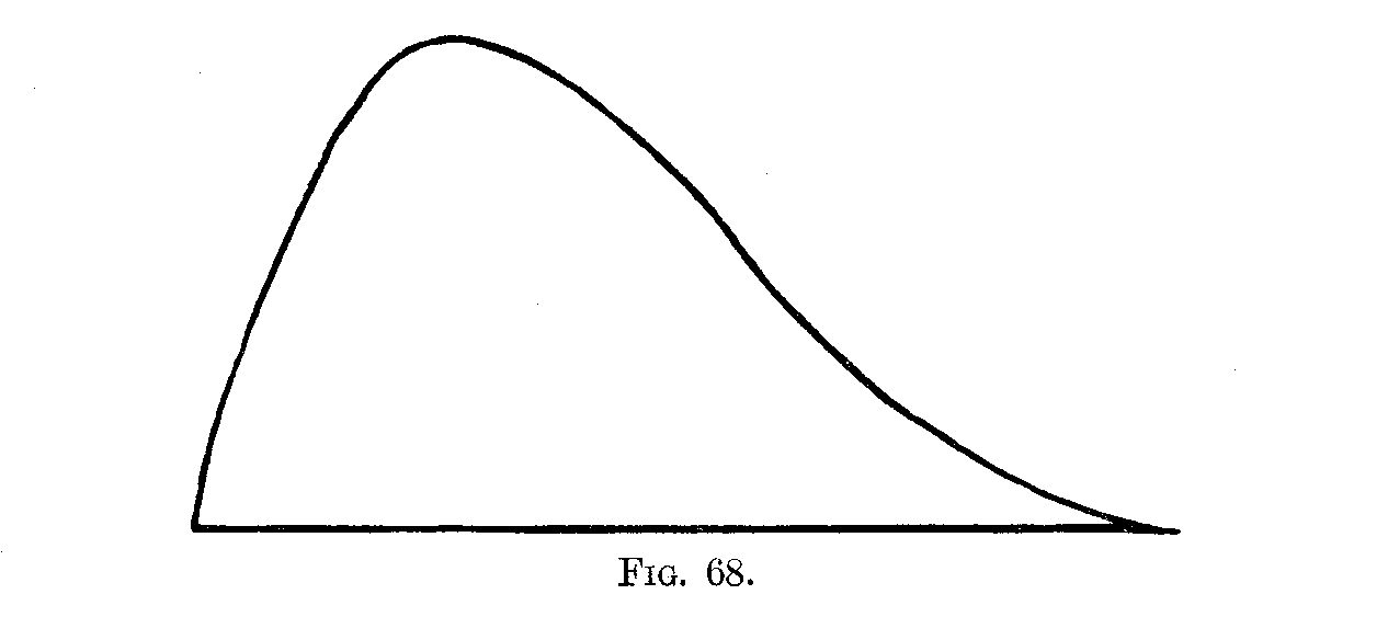
If a group of individuals are ranged in order according to the amounts which they severally possess of a trait, we can, even when ignorant of what the amounts are for each and all of the individuals, assign to each the amount of his deviation from the average, provided the form of the group's distribution is known. For instance, let 100 boys rank with respect to scholarship as shown below, and let the form of distribution be that of Fig. 68.
100 Boys—a, b, c, ETC.—RANKED BY RELATIVE POSITION
| a | is the highest ranking boy. |
| b, c, d | are next in rank and are rated equal. |
| e, f, g, h, i , j | are next in rank and are rated equal |
| k, l, m, n, o, p, q, r, s, t, | are next in rank and are rated equal |
| u, v, w, x, y, z, a, b, c, d, e, f, g, h, i | are next in rank and are rated equal |
| j, k, l, m, n, o, p, q, r, s, t, u, v, w, x, y, z | are next in rank and are rated equal |
| A, B, C, D, E, F, G, H, I, J, K, L, M, N, O, P, Q, R, S | are next in rank and are rated equal |
| T, U, V, W, X, Y, Z, α, β, γ, δ, ε, ζ, η | are next in rank and are rated equal |
| θ, ι, κ, λ, μ, ν, ξ, ο | are next in rank and are rated equal |
| π, ρ, σ, τ | are next in rank and are rated equal |
| υ, φ, χ | are next in rank and are rated equal |
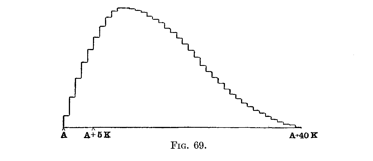
If we build up approximately the surface of Fig. 68 by a series of forty rectangles of equal base, the result is Fig. 69. This, the reader should observe, is done graphically by dividing the base line arbitrarily into forty equal parts, and by erecting a rectangle on each division of the base line—of such height that the mid-point
( 110) of its top is at the intersection of its top with the bounding line of the distribution of Fig. 68. There is no reason for the division of the base into forty rather than 60, or 70, or 120, equal parts.
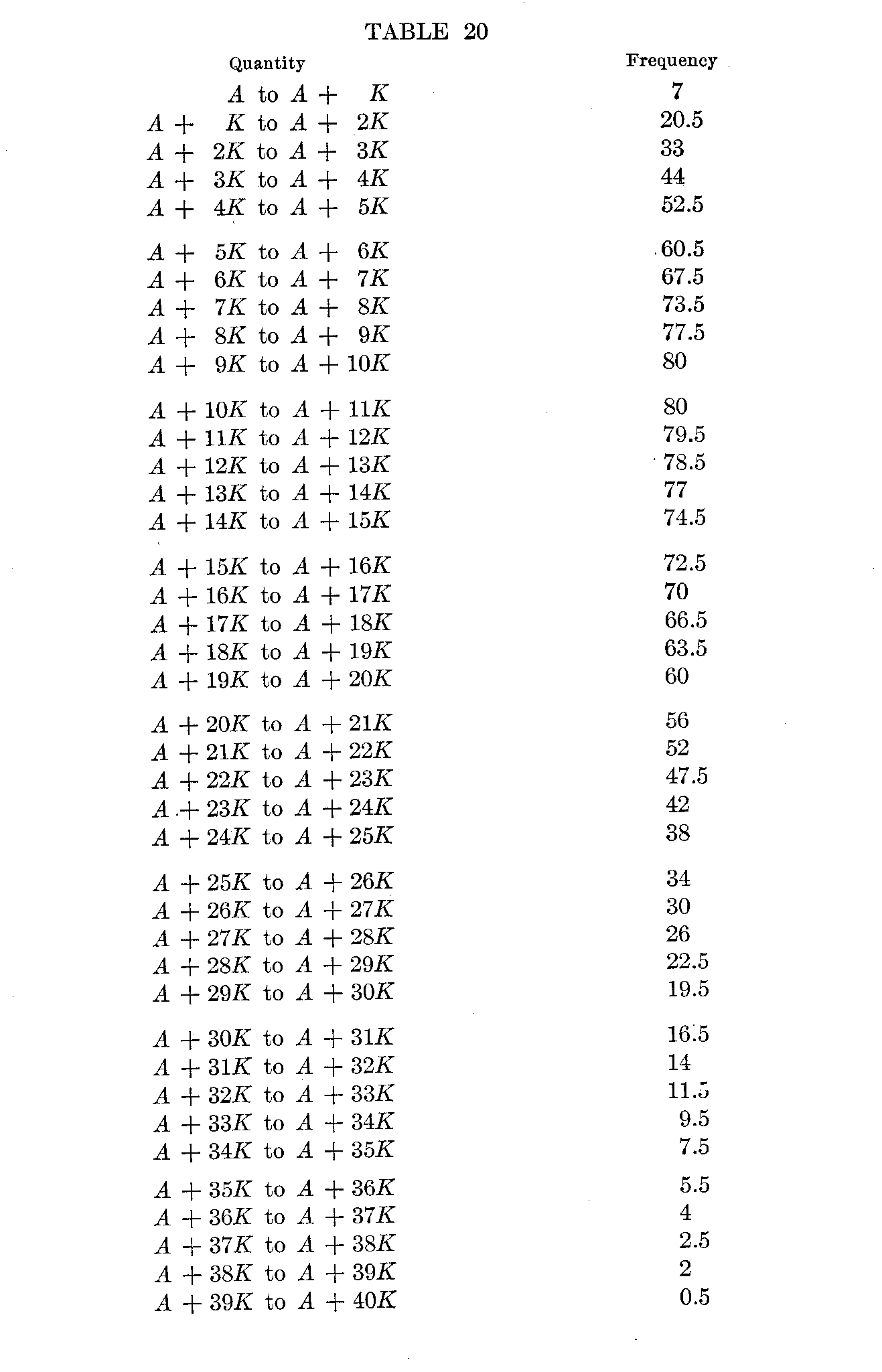
Call the distance of the low extreme from the absolute zero, A; and call the length of base of each of the rectangles, K. Then the upper extreme is at A + 40K, and the relative frequencies for the fortieths of the range—that is, the relative heights of the forty , rectangles—are as noted in Table 20, the total area being taken to be 1,680. These relative frequencies can, of course, be reckoned on the basis of any arbitrary value for the total area. There is no reason, save convenience, for assuming the area to be 1,680 rather than 2, 16,000, 1,820, or any other number. The 1,680 was an
accident of the particular scale used to measure the area of Fig. 69. If the
reader will construct an approximation made up of 60, or 80, or 100, rectangles,
and call the total area 1, 2, 500, 10,000 or any other number, he will still get
the same final values for the distances of a, b, c, d, etc., from any
defined point along the base-line, within
( 111) the range of the distribution, in terms of any defined feature of the distribution, say its range, A.D., a (S.D.), or Q.
(112)
This table of frequencies is like those hitherto described in this volume, save that two as yet unknown quantities, A and K, appear in the scale for quantity. This difference makes no difference in any formal respect. The table can be treated like any other. Thus its median is in the step "A + 14K to A + 15K," at approximately A + 14.12K. The mode may be taken as just between the steps, "A + 9K to A + 10K" and "A + 10K to A + 11K," or at A + 10K. The 25 percentile is at A + 8.8K. The 75 percentile is at A + 20.4K. 75 percentile — mode = 10.4K. Mode — 25 percentile = 1.2K. Q = 5.8K.
The highest-ranking boy, a, will then be represented by the 16.8 of the 1,680 frequency-units at the top, that is, toward A + 40K. His ability ranges from A + 40K to A + 34.7K (16.8 = 0.5 + 2.0 + 2.5 + 4 + 5.5 + 2.3; and 2.3 = .3 of 7.5).
The next three—b, c and d—will occupy the next 50.4 of the 1,680 frequency-units, and be included between the limits, A + 34.7K and A + 30.4K (7.5 - 2.3 = 5.2; 50.4 = 5.2 + 9.5 + 11.5 + 14.0 + 10.2; 10.2 = .6 of 16.5).
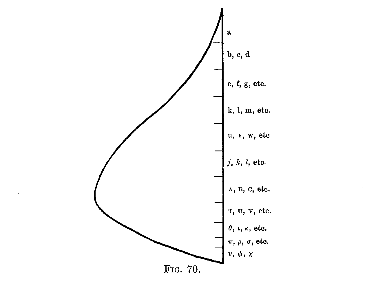
Similar calculations can be made for the next six—e, f, g, h, i and j—and so on. The results are shown graphically in Fig. 70.
( 113)
The average ability of each division may be calculated roughly from the facts obtained in this way. Thus the highest boy, a, being represented by 0.5 (A + 39.5K), 2 (A + 38.5K), 2.5 (A + 37.5K), 4 (A + 36.5K), 5.5 (A + 35.5K) and 2.3 (A + 34.5K),[1] has as an average A + 36.4K.[2]
A table can thus be formed as follows:
Boy a has as his approximate ability A + 36.4K;
Boys b, c, d have as their approximate ability A + 32.2K;[3]
Boys e, f, g, h, i, j have as their approximate ability A + 28.0K;
Boys k, 1, m, n, o, p, q, r, s, t have as their approximate ability A +
23.8K; etc.
So far we have defined or measured the scholarship of each boy as his distance above the low limit (A) of the whole group in terms of K as a unit. All of these measures can be turned into distances minus from the upper limit or plus and minus from the mode, average, median, or any other percentile point on the scale. They can be put in terms of any measure of the variability of the scheme, or of any part of it, instead of K. For instance, the best boy is + 36.4K or + 4.6Q from the mode.
The scholarship of every boy in the group can thus be represented in definite quantities of some unit of amount of difference K from some point of reference. This unit itself is definable as " the difference between this given person and that given person." The standard is similarly definable as the scholarship of such and such a given individual.
( 114)
By this method the obscurest and most complex traits, such as morality, enthusiasm, eminence, efficiency, courage, legal ability, inventiveness, etc., can be made material for ordinary statistical procedure, the one condition being that the general form of distribution of the trait in question be approximately known.
If now one has a group of individuals ranked by their relative position in the group, his first task before he can transmute the series of relative positions into a series of units of amount is to ascertain the form of distribution. This may be done (1) by measuring enough sample individuals objectively in units of amount, or (2) if the trait can not be measured in units of amount, by inferring the form of distribution from that of similar traits which can be.
1. Suppose one had 2,000 ten-year-old boys measured with respect to intellect by relative position.[4] If now one measured 200 of them objectively with tests scorable in units of amount, he could properly transmute the 2,000 on the basis of the type of distribution found for the 200.
2. Suppose one had 1,000 individuals measured with respect to delicacy of discrimination of sound by relative position. (It is well-nigh impossible to measure sensitiveness to sound in objective units which another observer can duplicate, because of the influence of size of room, resonance, etc.) It is fairly certain from studies of the delicacy of discrimination of length, weight, etc., that delicacy of discrimination of sound is distributed in something approximating sufficiently to a probability surface, with range of from + 3σ to � 3σ, to prevent calculations on that basis from being more than a little wrong on the average. We may, therefore, transmute the 1,000 measures by relative position into units of amount, on the hypothesis that such is the form of distribution.
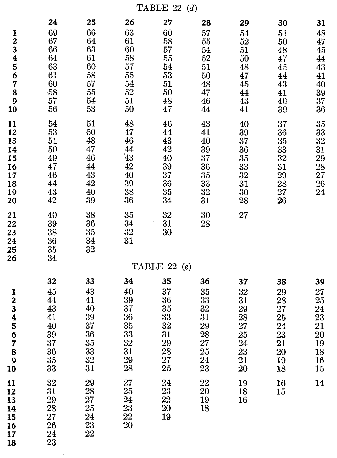
The labor of transmutation for cases which follow the probability type of distribution may be rendered almost nil by the use of tables. If the probability surface of range + 3σ to � 3σ is divided up into 100 equal areas representing the 100 successive per cents. from the highest to the lowest of the total group, and the average distance from the average in terms of σ is calculated for each per cent., the result is Table 21.
( 115)
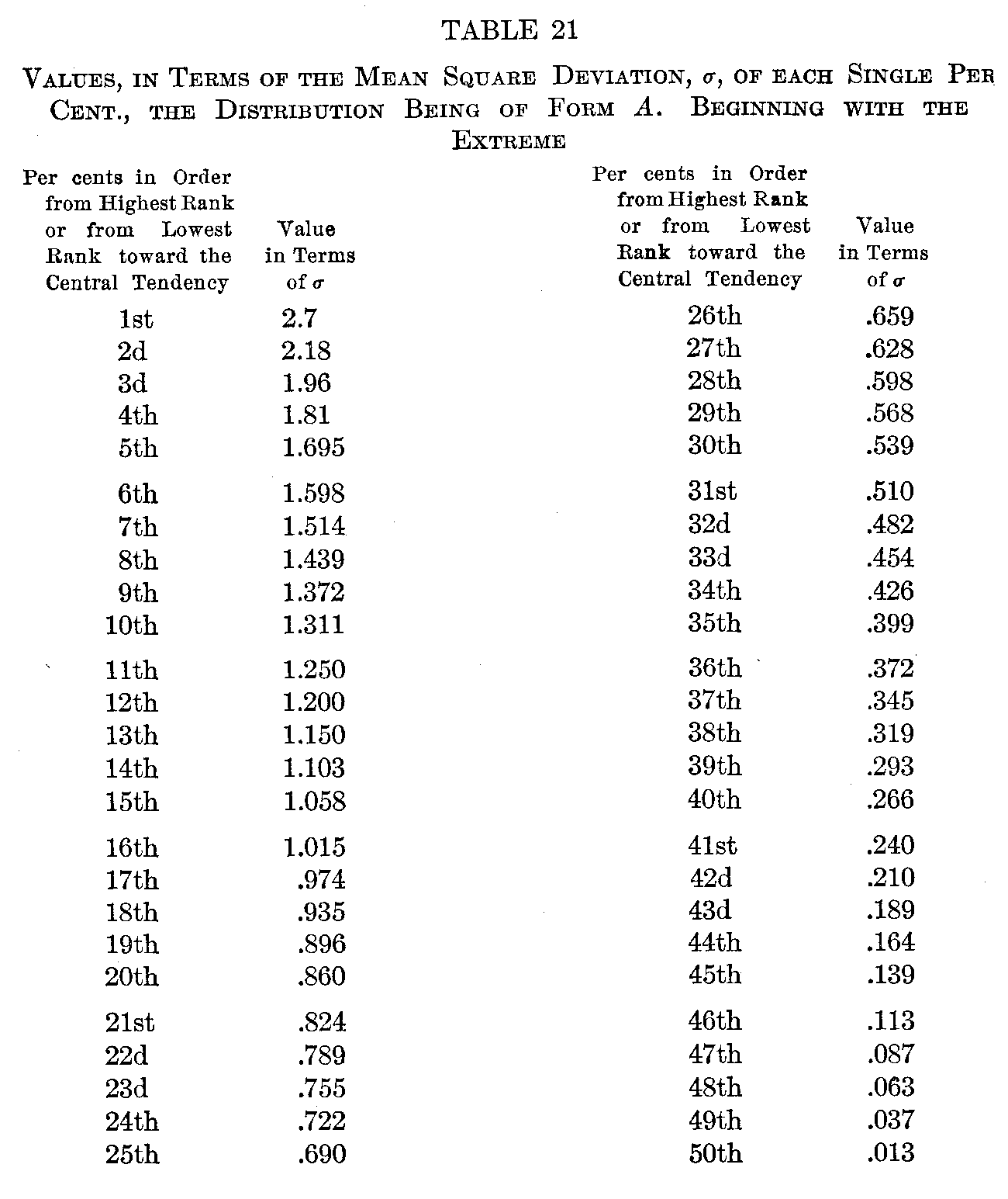
The figures along the top stand each for the percentage already made up in counting in from the extreme. The figures down the side stand for the percentage in the group for which a measure in
( 116) terms of amount is to be found. The entries in the body of the table stand for the average amount, in terms of σ, of any percentage counted in from any point toward the average. When a percentage passes the average (e. g., 30 per cent. after 40 per cent. have been used up in counting in from the top) it is necessary to take from the table two entries, one for the plus cases down to the average, the other for the minus cases, up to the average, of which the percentage is made up, and from these two entries to compute the average for the given percentage. Thus, 40 per cent. from the upper extreme having been used up, the next 30 per cent. will average
(+ .13 X 10) + (�.26 X 20)
13
or �.13.
Illustrations of the simpler usage in cases not passing the average are as follows:
The first 1 per cent. of a group averages + 2.7
The � 8 � �� � � average + 1.86
The 9th and 10th per cents of a group average+ 1.34
Per cents. 6, 7, and 8 from the bottom average �1.52
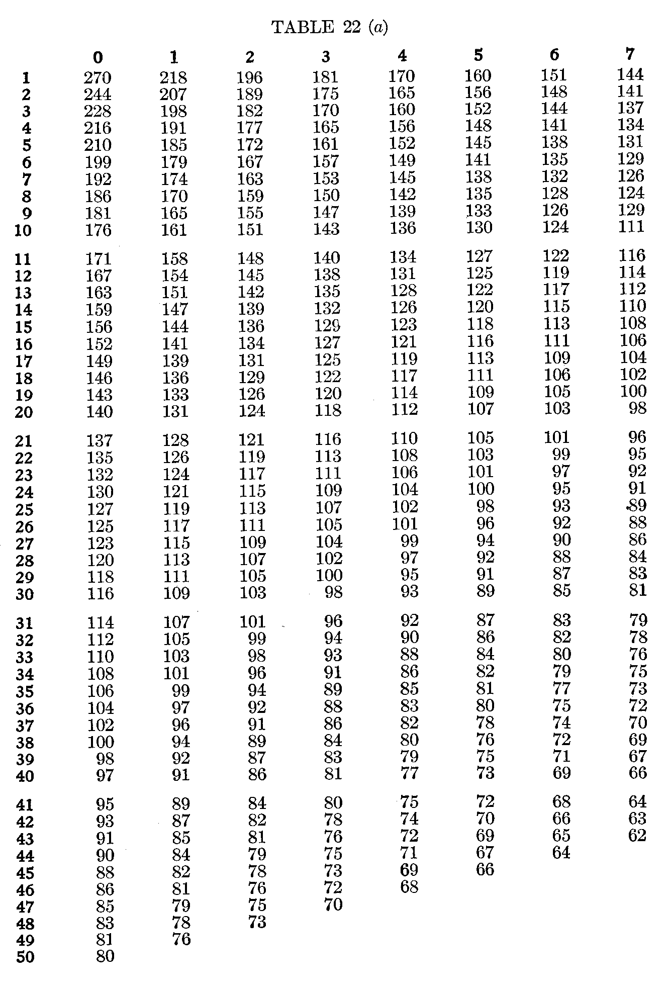
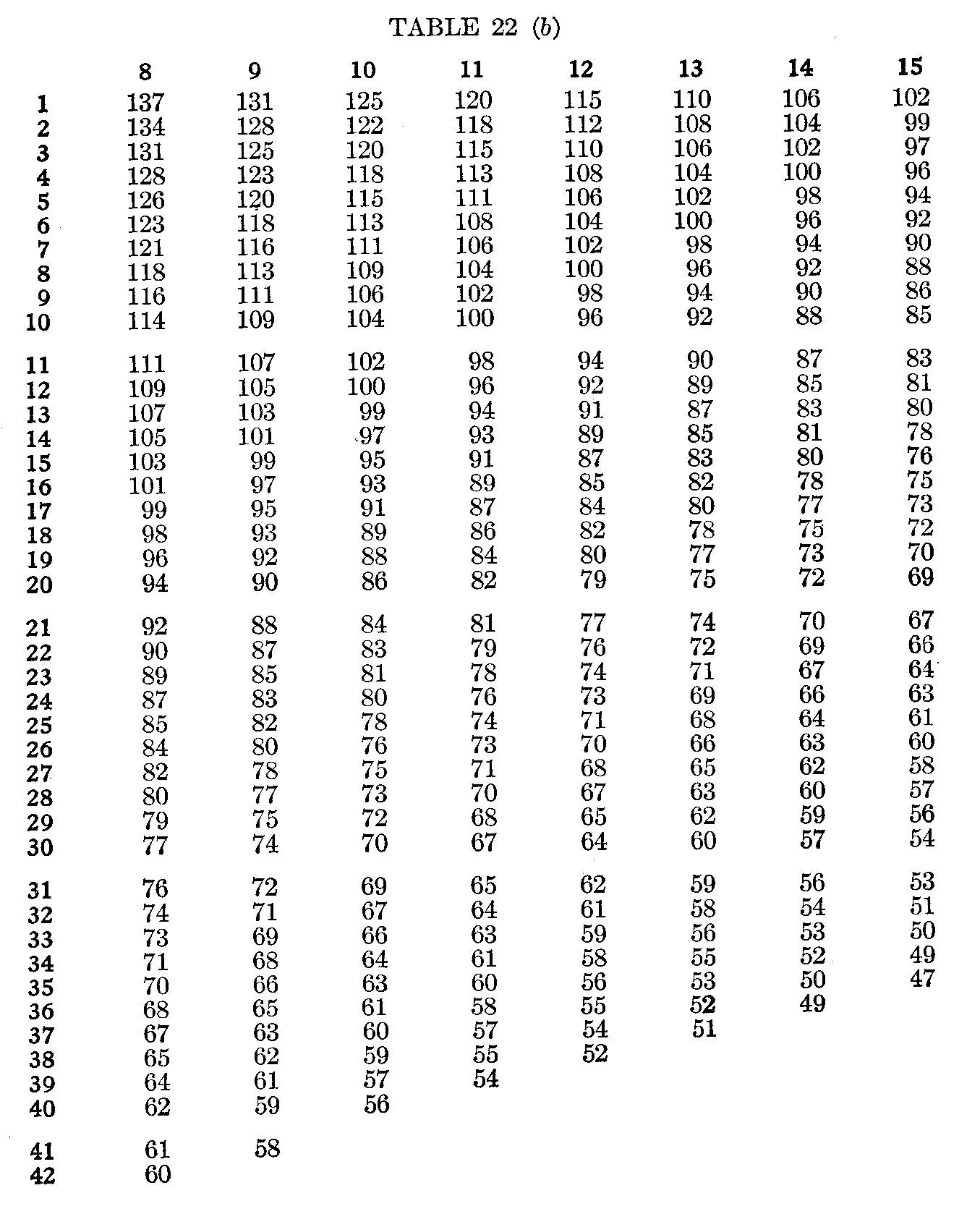
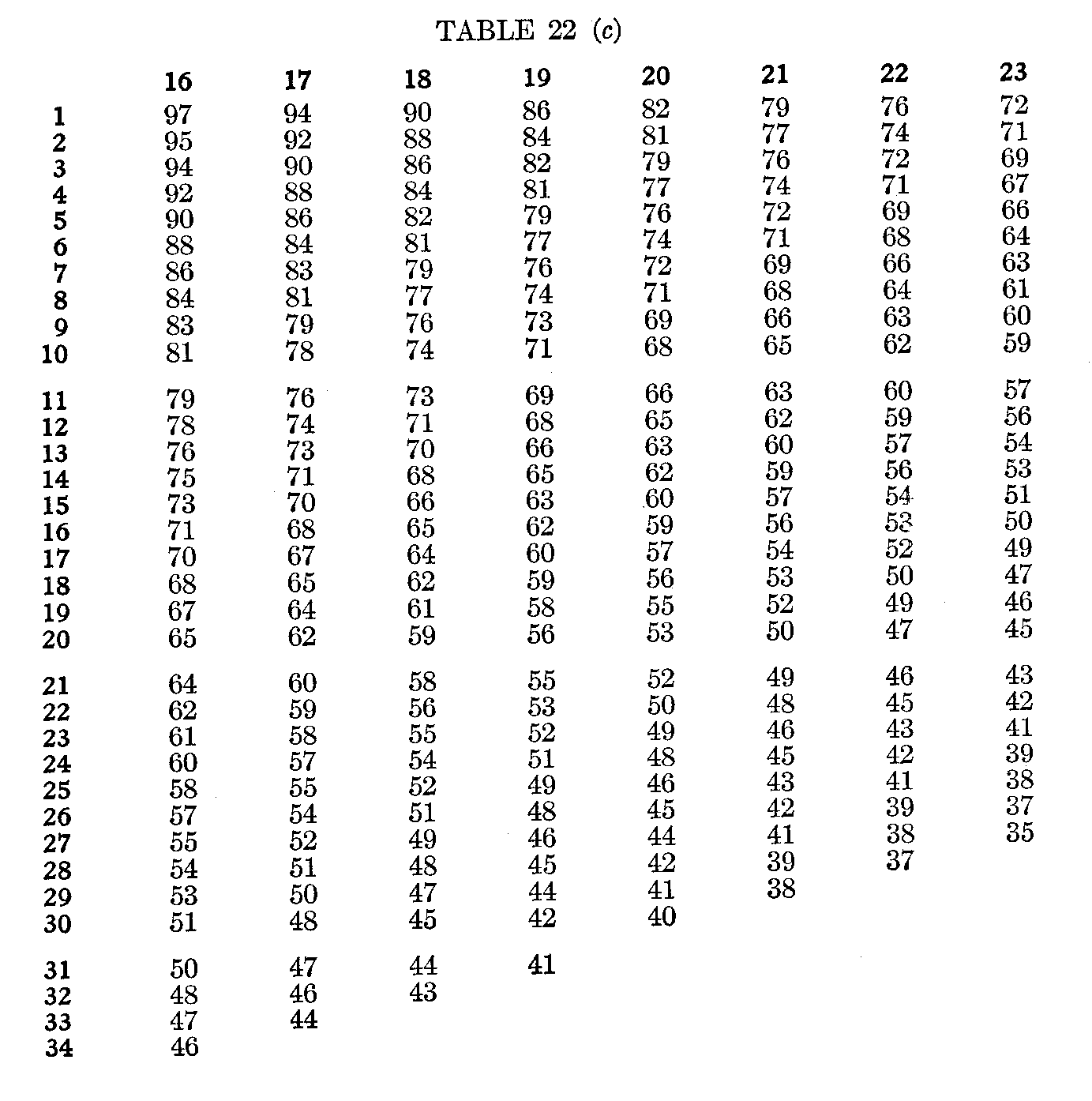
With the aid of Table 22 one can turn measurements by relative position into measurements in units of + or � σ almost as fast as one can read.
For instance, of 800 schoolboys,
8 per cent. received a mark of E
20 per cent. received a mark of VG
38 per cent. received a mark of G
24 per cent. received a mark of F
8 per cent. received a mark of P
2 per cent. received a mark of U
The table tells us at once that, in so far as the distribution of the ability in the group in question follows the form described above (Form A),
E = +1.86σ
VG = + .94σ
G = + .08e
F = � .80σ
P= � 1.59σ
U = � 2.44σ
( 117)
( 118)
( 119)
( 120)
(
121)
For any given form of distribution, a table like Table 22 can be constructed, by which any defined position in a series can be transmuted into terms of amount + or � from the mode, in units of the variability.
� 23. Transmutation by Means of Knowledge of the Equality of the Steps of Difference
The Equality of the Least Noticeable Difference.—There is still another possibility of turning measures by relative position into units of amount and so making them available for common scientific usage. In certain cases it may be justifiable to suppose that the least noticeable difference is a constant quantity for any one trait for any one observer; in simpler words, that if I say that John, James and Peter are to me indistinguishable, say, in literary merit, but that Henry and William are a shade better, and that George and Fred are a shade better than Henry and William, the actual difference between JJP and HW equals that between HW and GF. In so far as this were true, we could, with a large group of individuals varying continuously from the low to the high extreme, make groups on the basis of the least noticeable difference and call the steps of ability from group to group always the same.
The measures are then identical in form with those by ordinary units of amount. The only difference is that the amount of the quantity at the starting-point of the whole group (A) and the amount of the step from one subgroup to the next (K) are unknown except from the things measured themselves, and are undefinable except in terms of them. The question, "How much are A and K?" can be answered only by pointing to the achievements of the lowest group and saying, "That is A," by pointing to the differences be-
( 122) -tween that group and others and saying, "This much difference is K, this much 4K, this much 20K and so on," K being the least noticeable difference.
The hypothesis that the least noticeable difference in a trait is for the same observer a constant quantity has not been tested sufficiently to decide how far its use is justifiable, but there can be no doubt that some modification of the principle involved will some time be a valuable resource of the theory of mental measurements.
The Equality of Equally Often Noticed Differences.—Suppose specimens a, b, c, d, e, f, etc., to be ranked in order for trait X a hundred times. The hundred rankings may comprise a hundred judgments by one judge, or one judgment by each of a hundred judges, or ten judgments by each of ten judges, etc., etc., without alteration in the general procedure. Suppose that a is placed below b 74 times, and above b 26 times; suppose that b is placed below c 74 times, and above c 26 times; suppose that c is placed below d 74 times, and above d 26 times. Then if "equally often noticed" can be assumed to mean equal," the differences, b — a, c — b, and d — c, are equal. Let A = the difference between the amount of trait X possessed by a and the absolute zero for X. Let K = the amount of difference which the observer in question notices 74 times out of a hundred. Then the measure of a is A; that of b is A + K; that of c is A + 2K, etc. The measures are now identical in form with those by ordinary units of amount. For this method to be applicable, the percentage of observations of a difference must be less than 100, since if two differences are always noticed, one may be very small and one very great. The method as a whole presupposes that the observations are made by judges of some competence. Its precision depends upon how competent they are.
� 24. Transmutation by Means of the Amount of Agreement of Different Judges in Respect to the Relative Positions
Suppose that, in the case quoted in Section 23, the percentages of judgments of difference had been:
a below b,74
b below c,74
c below d,74
( 123)
d below e,70
e below f,
80
f below g,
60
g below h,90
Now, for the same reasons which make it allowable, the judges being competent, to infer equality in the differences b — a, c — b and d — c, we can infer that e — d and g — f are less than b — a, c — b and d — c; and can infer that f — e and h — g are greater than b — a, c — b, and d — c. We can infer, that is, that (h — g) > (f—e)> (b — a) = (c—b)= (d—c)> (e—d)> (g — f).
It is possible, by making a further assumption, to infer how much greater g — h is than e — f, and so on for the other differences in the series. The assumption to be made concerns the relation between the amount of a difference and the percentage of times that it will be noticed. The theories at the basis of any such assumptions are beyond the scope of this book, but the probably best relation to assume is that shown in Table 23. In this table, 1.00 is taken arbitrarily to equal such a difference between two facts, a and b, that b will be judged > a in 75 per cent. of the judgments and < a in 25 per cent. of the judgments. That is, 1.00, or b — a, is positive; and is the amount of difference whose direction is noted correctly in 75 per cent. of the judgments. If then the fact q is judged greater than p in 51 per cent. of the judgments, q — p, by the table equals .04; if w is judged greater than v in 52 per cent. of the judgments, w — v = .07; and so on through the table.
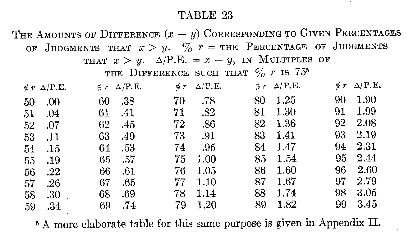
(124)
In our illustrative case, we have, from Table 23:
b—a=.95
c—b= .95
d—e= .95
e—d= .78
f — e = 1.25
g—f= .38
h — g = 1.90
and, letting A equal the difference between a and the absolute zero for the trait in question,
a=A
b=A+.95
c =A +1.90
d=A+2.85
e = A + 3.63
f =A+4.88
g = A + 5.26
h = A + 7.16
wherein 1.00 equals a difference a trifle greater than b — a, c — b, or d — e, or such a difference as 75 per cent. of the judgments in question would note correctly.
For reasons not to be stated here it is best to avoid relying on this table outside the limits of 65 and 85 for the percentages of judgments that one fact is greater or less than another (per cent. r).
PROBLEMS
29. Using Table 21, calculate the measure in terms of units of amount: (1) of the highest four per cent. of a group normally distributed; (2) of the six per cent. just above the mode; (3) of the three per cent. from the end of the seventeenth down—that is, of the 18th, 19th and 20th per cents. Verify the results from the entries for these groups in Table 22.
30. Construct the beginning of a table like Table 22 for the form of distribution (Form D) shown in Fig. 23 and Table 11, putting in the entries for percentages 1, 2, 3, 4 and 5, for each of the three cases of 0, 1 %, and 2 % already used. Begin at the extreme of greater skewness. Be accurate to the first decimal (tenths of a).
31. Suppose 100 individuals to be ranked in order as follows:
a is the best
b, c, d, e are the next, and are
indistinguishable in merit.
f, g, h, j
are
the next, and are indistinguishable in merit.
k, 1, m, n, o
p, q, r, s, t are the next, and are indistinguishable in merit.
etc, etc.
Supply the approximate values in the following:
a is + _Q from the median if the distribution is a rectangle.
b is + _Q from the median if the distribution is a rectangle.
f is + _Q from the median if the distribution is a rectangle.
s is + _Q from the median if the distribution is a rectangle.
a is + _σ from the median or Av. if the distribution is of Form A.
b is + _σ from the median or Av. if the distribution is of Form A.
f is + _σ from the median or Av. if the distribution is of Form A.
s is + _σ from the median or Av. if the distribution is of Form A.
a is + _σ from the mode if the distribution is of Form D.
b is + _σ from the mode if the distribution is of Form D.
32. On the hypothesis that the distribution of darkness of eyes is of Form A, use Table 22 and transmute into terms of units of amount the following measures by relative position:
Eye ColorPer Cents. of Englishman
[6]
Light blue
2.9 call 3
Blue. Dark blue 29.3 call 29
Gray. Blue green 30.2 call 30
Dark gray. Hazel 12.3 call 12
Light brown. Brown
11.0 call 11
Dark brown
10.8 call 11
Very dark brown. Black 3.6 call 4
It is possible, by interpolating, to use the table for a finer scale than to a single per cent. But it is hardly worth while.
33. Suppose a group of individuals to receive grades as follows in a trait in which variation is continuous: 2 per cent. received A; 22 per cent. received B; 44 per cent. received C; 25 per cent. received D; 6 per cent. received E; 1 per cent. received F. Suppose that this grouping is by equally often noticed differences and that the differences can be assumed equal. Calculate the approximate values to complete the following:
a grade of A = _Q from the Median.
a grade of B = _Q from the Median.
a grade of C = _Q from the Median.
a grade of D = _Q from the Median.
a grade of E = _Q from the Median.
a grade of F = _Q from the Median.
34. Suppose that a certain man, Z, whose life was fully known, was, by the average opinion of a hundred statesmen, scientists and men of general wisdom, rated as having just barely contributed a
( 126) balance of one trivial satisfaction to a balance of one person in the world, past, present and future. Suppose that by the same hundred expert judges of the services performed by human individuals, we have the lives of twenty-five men, Y, X, W, V, etc., up to A, A being Pasteur, rated as having performed services such that A — B, B — C, C — D, D — E, etc., are all equal.
Suppose that you knew the lives of two men—a and b. How would you answer the question: How many times as great was a's service to the world as b's? Under what conditions would your answer be true? What factors would work to make it depart from the truth?